前言:
牛奶冻曲线(blancmange curve),因在1901年由高木贞治所研究,又称高木曲线。
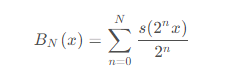
在单位区间内,牛奶冻函数定义为:

分形曲线的轮廓会随着阶数的增多而填充细节,即对于下面的 来说, N的变化会增添曲线的自相似特性
import numpy as np
import matplotlib.pyplot as plt
s = lambda x : np.min([x-np.floor(x), np.ceil(x)-x],0)
x = np.arange(1000).reshape(-1,1)/1000
N = np.arange(30).reshape(1,-1)      #2^N已经很大了,精度足够
b = np.sum(s(2**N*x)/2**N,1)
plt.plot(b)
plt.show()
如图所示:

牛奶冻曲线是一种典型的分形曲线,即随着区间的不断缩小,其形状几乎不发生什么变化,例如更改自变量的范围,令
x = np.arange(0.25,0.5,1e-3).reshape(-1,1)
最终得到的牛奶冻曲线在观感上是没什么区别的。
接下来绘制一下,当区间发生变化时,牛奶冻曲线的变化过程
绘图代码为:
from aniDraw import *

# 三角波函数
s = lambda x : min(np.ceil(x)-x, x-np.floor(x))
s = lambda x : np.min([x-np.floor(x), np.ceil(x)-x],0)
x = np.arange(1000).reshape(-1,1)/1000
N = np.arange(30).reshape(1,-1)      #2^N已经很大了,精度足够
b = np.sum(s(2**N*x)/2**N,1)
fig = plt.figure(figsize=(12,8))
ax = fig.add_subplot()
# n为坐标轴参数
def bcFunc(n):
    st = 1/3 - (1/3)**n
    ed = 1/3   (2/3)**n
    x = np.linspace(st,ed,1000).reshape(-1,1)
    b = np.sum(s(2**N*x)/2**N,1)
    return (x,b)

line, = ax.plot([],[],lw=1)

def animate(n):
    x,y = bcFunc(n)
    line.set_data(x,y)
    plt.xlim(x[0],x[-1])
    plt.ylim(np.min(y),np.max(y))
    return line,

Ns = np.arange(1,10,0.1)
ani = animation.FuncAnimation(fig, animate, Ns,
    interval=125, blit=False)
plt.show()
到此这篇关于Python绘制牛奶冻曲线(高木曲线)案例的文章就介绍到这了,更多相关Python 牛奶冻曲线内容请搜索Devmax以前的文章或继续浏览下面的相关文章希望大家以后多多支持Devmax!